问题
在 Transformer 之前,在 RNN 之前,在词向量之前,语言模型通过统计「下一个词跟在之前 n-1 个词后面的频率」来预测下一个词。数一数 "the cat" → "sat" 出现 47 次,"the cat" → "jumped" 出现 12 次,"the cat" → "refrigerator" 出现 0 次。归一化后得到概率分布。
这就是 n-gram 语言模型。从 1980 年到 2015 年,它驱动了每一个语音识别器、每一个拼写检查器和每一个基于短语的机器翻译系统。当你需要廉价、设备端的语言建模时,它仍在运行。
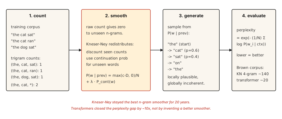
有意思的问题是:如何处理没见过的 n-gram。原始计数模型会给任何没见过的序列分配零概率,这是灾难性的,因为句子很长,而几乎每个长句都至少包含一个没见过的序列。五十年的平滑研究解决了这个问题。Kneser-Ney 平滑是其成果,现代深度学习继承了其实证传统。
概念
预测游戏
在这套机制出现之前,一个实验定义了什么是语言模型。遮住英文句子的下一个字母。请人来猜,一次一个,直到猜对。记下猜测次数。重复几百个字母。
这些猜测次数不是琐碎之事。它们是文本的无损重编码:把次数序列交给第二个相同的猜测者,他们能重建每个字母,因为在每个位置他们确切知道哪些猜测排在前头。一个能用更少符号重编码的消息,每个符号携带的信息更少,因此猜测次数统计给出了英语熵的上界。
Shannon 在 1951 年做了这个实验,得到的数字至今仍支配着这个领域。27 个符号的字母表(26 个字母加空格)每个字母可携带 log2(27) ≈ 4.75 比特。有 100 个字母上下文的人类猜测者落在每字母 0.6 到 1.3 比特之间。英语大约四分之三是被锁定(forced moves)。模型必须学习的结构,在任何模型能学习它之前就被测量出来了。
此后的每个语言模型都是这个游戏的机械玩家,本课里的每个评估数字都是这个游戏的得分:
- 交叉熵损失是模型每个符号平均需要的比特数。训练 LM 字面上就是最小化它在猜词游戏中的得分。
- 困惑度是
2^bits(或e^nats):模型在猜测之后仍面临的分支因子。在 27 个符号上均匀猜测的困惑度是 27;每字母 1 比特的玩家困惑度是 2。 - 上下文长度是玩家的记忆。 trigram 模型用两个 token 的记忆玩。Transformer 用 100K token 玩同一个游戏。规则从未改变;玩家变强了。
有一个单位切换要留意:游戏按字母以比特(log2)计分,而下文的 n-gram 公式按词 token 以 nat(自然对数)计分——由于以 nat 计的困惑度 e^H 等于以比特计的 2^H,两种视角是用不同单位表达的同一种测量。
N-gram 概率: P(w_i | w_{i-n+1}, ..., w_{i-1})。固定 n(通常 trigram 取 3,4-gram 取 4)。由计数计算:
零计数问题。 训练中没见过的任何 n-gram 概率为零。2007 年一项针对 Brown 语料库的研究发现,即使 4-gram 模型,留出的 4-gram 中也有 30% 在训练中未见过。不做平滑,你无法在任何真实文本上评估。
平滑方法,按复杂程度排序:
- Laplace(加一)。 给每个计数加 1。简单,对稀有事件效果很差。
- Good-Turing。 根据频次之频次(frequency-of-frequencies),把概率质量从高频事件重新分配给未见事件。
- 插值(Interpolation)。 用可调权重组合 n-gram、(n-1)-gram 等估计。
- 回退(Backoff)。 如果 n-gram 计数为零,回退到 (n-1)-gram。Katz 回退对此做归一化。
- 绝对折扣(Absolute discounting)。 从所有计数中减去固定折扣
D,重新分配给未见事件。 - Kneser-Ney。 绝对折扣,加上对低阶模型的巧妙选择:使用延续概率(一个词出现在多少个上下文中)而不是原始频率。
Kneser-Ney 的洞见很深。"San Francisco" 是常见的 bigram。unigram "Francisco" 大多出现在 "San" 之后。朴素的绝对折扣给 "Francisco" 很高的 unigram 概率(因为计数高)。Kneser-Ney 注意到 "Francisco" 只出现在一个上下文中,于是相应降低它的延续概率。结果:以 "Francisco" 结尾的新 bigram 得到恰当的低概率。
评估:困惑度。 留出测试集上每个词平均负对数似然的指数。越低越好。困惑度 100 意味着模型的困惑程度相当于在 100 个词中均匀选择。
构建它
第 1 步:trigram 计数
pythonfrom collections import Counter, defaultdict
def train_ngram(corpus_tokens, n=3):
ngrams = Counter()
contexts = Counter()
for sentence in corpus_tokens:
padded = ["<s>"] * (n - 1) + sentence + ["</s>"]
for i in range(len(padded) - n + 1):
ctx = tuple(padded[i:i + n - 1])
word = padded[i + n - 1]
ngrams[ctx + (word,)] += 1
contexts[ctx] += 1
return ngrams, contexts
def raw_probability(ngrams, contexts, context, word):
ctx = tuple(context)
if contexts.get(ctx, 0) == 0:
return 0.0
return ngrams.get(ctx + (word,), 0) / contexts[ctx]输入是已分词的句子列表。输出是 n-gram 计数和上下文计数。<s> 和 </s> 是句子边界。
第 2 步:Laplace 平滑
pythondef laplace_probability(ngrams, contexts, vocab_size, context, word):
ctx = tuple(context)
numerator = ngrams.get(ctx + (word,), 0) + 1
denominator = contexts.get(ctx, 0) + vocab_size
return numerator / denominator给每个计数加 1。能平滑,但给未见事件分配了过多质量,也损害了稀有但已知的事件。
第 3 步:Kneser-Ney(bigram,插值)
pythondef kneser_ney_bigram_model(corpus_tokens, discount=0.75):
unigrams = Counter()
bigrams = Counter()
unigram_contexts = defaultdict(set)
for sentence in corpus_tokens:
padded = ["<s>"] + sentence + ["</s>"]
for i, w in enumerate(padded):
unigrams[w] += 1
if i > 0:
prev = padded[i - 1]
bigrams[(prev, w)] += 1
unigram_contexts[w].add(prev)
total_unique_bigrams = sum(len(ctx_set) for ctx_set in unigram_contexts.values())
continuation_prob = {
w: len(ctx_set) / total_unique_bigrams for w, ctx_set in unigram_contexts.items()
}
context_totals = Counter()
for (prev, w), count in bigrams.items():
context_totals[prev] += count
unique_follow = defaultdict(set)
for (prev, w) in bigrams:
unique_follow[prev].add(w)
def prob(prev, w):
count = bigrams.get((prev, w), 0)
denom = context_totals.get(prev, 0)
if denom == 0:
return continuation_prob.get(w, 1e-9)
first_term = max(count - discount, 0) / denom
lambda_prev = discount * len(unique_follow[prev]) / denom
return first_term + lambda_prev * continuation_prob.get(w, 1e-9)
return prob三个活动部件。continuation_prob 捕捉「这个词出现在多少个不同的上下文中?」(Kneser-Ney 的创新)。lambda_prev 是折扣释放出的质量,用来给回退加权。最终概率是折扣主项加上加权的延续项。
第 4 步:用采样生成文本
pythonimport random
def generate(prob_fn, vocab, prefix, max_len=30, seed=0):
rng = random.Random(seed)
tokens = list(prefix)
for _ in range(max_len):
candidates = [(w, prob_fn(tokens[-1], w)) for w in vocab]
total = sum(p for _, p in candidates)
r = rng.random() * total
acc = 0.0
for w, p in candidates:
acc += p
if r <= acc:
tokens.append(w)
break
if tokens[-1] == "</s>":
break
return tokens按概率成比例采样。每个随机种子总得到不同输出。想要类似束搜索的输出,就在每步取 argmax(贪心),并加一个小随机性旋钮(温度)。
第 5 步:困惑度
pythonimport math
def perplexity(prob_fn, sentences):
total_log_prob = 0.0
total_tokens = 0
for sentence in sentences:
padded = ["<s>"] + sentence + ["</s>"]
for i in range(1, len(padded)):
p = prob_fn(padded[i - 1], padded[i])
total_log_prob += math.log(max(p, 1e-12))
total_tokens += 1
return math.exp(-total_log_prob / total_tokens)越低越好。对 Brown 语料库,调好的 4-gram KN 模型困惑度在 140 左右。Transformer LM 在同一测试集上达到 15-30。差距约为 10 倍。这个差距正是领域继续前进的原因。
使用它
- 经典 NLP 教学。 你能获得的对平滑、MLE 和困惑度最清晰的介绍。
- KenLM。 生产级 n-gram 库。用作语音和 MT 系统中对延迟敏感的重新打分器。
- 设备端自动补全。 键盘里的 trigram 模型。今天仍是如此。
- 基线。 在宣称你的神经 LM 很好之前,务必先算一个 n-gram LM 困惑度。如果你的 Transformer 没有大幅超过 KN,一定有问题。
交付它
保存为 outputs/prompt-lm-baseline.md:
markdown---
name: lm-baseline
description: Build a reproducible n-gram language model baseline before training a neural LM.
phase: 5
lesson: 16
---
Given a corpus and target use (next-word prediction, rescoring, perplexity baseline), output:
1. N-gram order. Trigram for general English, 4-gram if corpus is large, 5-gram for speech rescoring.
2. Smoothing. Modified Kneser-Ney is the default; Laplace only for teaching.
3. Library. `kenlm` for production, `nltk.lm` for teaching, roll your own only to learn.
4. Evaluation. Held-out perplexity with consistent tokenization between train and test sets.
Refuse to report perplexity computed with different tokenization between systems being compared — perplexity numbers are comparable only under identical tokenization. Flag OOV rate in test set; KN handles OOV poorly unless you reserve a special <UNK> token during training.练习
- 简单。 在一个 1,000 句的莎士比亚语料上训练 trigram LM。生成 20 个句子。它们在局部看似合理,在全局却不连贯。这是经典演示。
- 中等。 在留出的莎士比亚切分上为你的 KN 模型实现困惑度。与 Laplace 比较。你应该看到 KN 的困惑度低 30-50%。
- 困难。 构建一个 trigram 拼写纠正器:给定拼错的词及其上下文,生成候选纠正并按 LM 下的上下文概率排序。在 Birkbeck 拼写语料库(公开)上评估。
关键术语
| 术语 | 人们怎么说 | 实际含义 |
|---|---|---|
| N-gram | 词序列 | n 个连续 token 的序列。 |
| Smoothing | 避免零 | 重新分配概率质量,使未见事件得到非零概率。 |
| Perplexity | LM 质量指标 | 留出数据上的 exp(-average log-prob)。越低越好。 |
| Backoff | 回退到更短上下文 | 如果 trigram 计数为零,就用 bigram。Katz 回退将其形式化。 |
| Kneser-Ney | n-gram 的最佳平滑 | 绝对折扣 + 低阶模型的延续概率。 |
| Continuation probability | KN 特有 | P(w) 按 w 出现的上下文数加权,而不是按原始计数。 |
| Entropy of text | 每符号的信息量 | 给定上下文编码下一个符号平均所需的比特数。Shannon 1951 年对印刷英语(最多 100 个字母上下文)的估计:每字母 0.6-1.3 比特,在任何模型出现之前测得。 |
延伸阅读
- Shannon (1951). Prediction and Entropy of Printed English —— 定义了每个语言模型至今仍在优化的目标的猜词游戏实验。
- Jurafsky and Martin — Speech and Language Processing, Chapter 3 (2026 draft) —— 关于 n-gram LM 和平滑的权威论述。
- Chen and Goodman (1998). An Empirical Study of Smoothing Techniques for Language Modeling —— 确立 Kneser-Ney 为最佳 n-gram 平滑器的论文。
- Kneser and Ney (1995). Improved Backing-off for M-gram Language Modeling —— 原始 KN 论文。
- KenLM —— 快速的生产级 n-gram LM,2026 年仍用于延迟敏感的应用。
示意图共 1 张