The Problem
VAEs produce blurry samples because their MSE decoder loss is Bayes-optimal for the mean image — and the mean of many plausible digits is a fuzzy digit. You want a loss that rewards plausibility, not pixel-wise proximity to any one target. There is no closed-form for plausibility. You have to learn it.
Goodfellow's idea: train a classifier D(x) to distinguish real images from fakes. Train a generator G(z) to fool D. The loss signal for G is whatever D currently thinks makes something look real. This signal updates as G improves, chasing a moving target. If both networks converge, G has learned the data distribution without ever writing down log p(x).
This is adversarial training. The math is a minimax game:
In 2026 GANs are no longer the SOTA generator (diffusion and flow matching ate that crown). But StyleGAN 2/3 remain the sharpest face models ever shipped, GAN discriminators are used as perceptual losses in diffusion training, and adversarial training powers the fast 1-step distillations (SDXL-Turbo, SD3-Turbo, LCM) that let you ship real-time diffusion.
The Concept
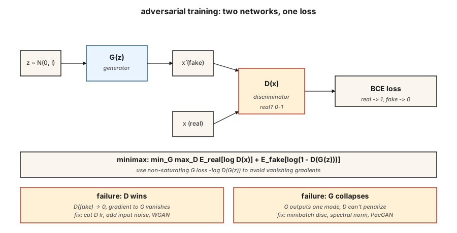
Generator G(z). Maps a noise vector z \sim \mathcal{N}(0, I) to a sample \hat{x}. A decoder-shaped network (dense or transposed conv).
Discriminator D(x). Maps a sample to a scalar probability (or score). Real → 1, fake → 0.
Loss. Two alternating updates:
- Train D: \text{loss}_D = -[ \log D(x) + \log(1 - D(G(z))) ]. Binary cross-entropy on real=1, fake=0.
- Train G: \text{loss}_G = -\log D(G(z)). This is the non-saturating form Goodfellow used (original \log(1 - D(G(z))) saturates and kills gradients when D is confident).
Training loop. One step of D, one step of G. Repeat.
Why it works. If G perfectly matches p_{\text{data}}, then D cannot do better than chance and outputs 0.5 everywhere; G gets no more gradient. Equilibrium.
Why it breaks. Mode collapse (G finds one mode D can't classify and mints it forever), vanishing gradient (D learns too fast and \log D saturates), training instability (learning rates, batch sizes, anything).
Variants that made GANs work
| Year | Innovation | Fix |
|---|---|---|
| 2015 | DCGAN | Conv/deconv, batch norm, LeakyReLU — the first stable architecture. |
| 2017 | WGAN, WGAN-GP | Replace BCE with Wasserstein distance + gradient penalty. Fixes vanishing gradient. |
| 2017 | Spectral normalization | Lipschitz-bound the discriminator. Still used in 2026 discriminators. |
| 2018 | Progressive GAN | Train low-res first, add layers. First megapixel results. |
| 2019 | StyleGAN / StyleGAN2 | Mapping network + adaptive instance norm. State of the art for fixed-domain photorealism. |
| 2021 | StyleGAN3 | Alias-free, translation-equivariant — still the face gold standard in 2026. |
| 2022 | StyleGAN-XL | Conditional, class-aware, larger scale. |
| 2024 | R3GAN | Rebrands with stronger regularization; works on 1024² without tricks. |
Build It
code/main.py trains a tiny GAN on 1-D data: a mixture of two Gaussians. Generator and discriminator are single-hidden-layer MLPs. We implement forward, backward, and the minimax loop by hand. The goal is to see the two key failure modes (mode collapse + vanishing gradient) as they happen.
Step 1: non-saturating loss
The vanilla Goodfellow loss \log(1 - D(G(z))) goes to 0 when D classifies G's fake as fake with high confidence. At that point the gradient for G is basically zero — G cannot improve. The non-saturating form -\log D(G(z)) has the opposite asymptote: it blows up when D is confident, giving G a strong signal.
pythondef g_loss(d_fake):
# maximize log D(G(z)) <=> minimize -log D(G(z))
return -sum(math.log(max(p, 1e-8)) for p in d_fake) / len(d_fake)Step 2: one discriminator step per generator step
pythonfor step in range(steps):
# train D
real_batch = sample_real(batch_size)
fake_batch = [G(z) for z in sample_noise(batch_size)]
update_D(real_batch, fake_batch)
# train G
fake_batch = [G(z) for z in sample_noise(batch_size)] # fresh fakes
update_G(fake_batch)Fresh fakes for G, otherwise gradients are stale.
Step 3: watch for mode collapse
pythonif step % 200 == 0:
samples = [G(z) for z in sample_noise(500)]
mode_a = sum(1 for s in samples if s < 0)
mode_b = 500 - mode_a
if min(mode_a, mode_b) < 50:
print(" [!] mode collapse: one mode is starved")The canonical symptom: one of the two real modes stops being generated. The discriminator stops correcting it because it's never seen as a fake.
Pitfalls
- Discriminator too strong. Cut D's learning rate by 2-5x, or add instance/layer noise. If D reaches >95% accuracy, G is dead.
- Generator memorizes a mode. Add noise to D inputs, use a minibatch-discriminator layer, or switch to WGAN-GP.
- Batch norm leaking statistics. Real batch + fake batch flowing through the same BN layer mixes their statistics. Use instance norm or spectral norm instead.
- Inception-score gaming. FID and IS are noisy at low sample counts. Use ≥10k samples at eval.
- One-shot sampling is a lie for conditional tasks. You still need CFG scales, truncation tricks, and re-sampling to get usable outputs.
Use It
The 2026 GAN stack:
| Situation | Pick |
|---|---|
| Photoreal human faces, fixed pose | StyleGAN3 (sharpest, smallest) |
| Anime / stylized faces | StyleGAN-XL or Stable Diffusion LoRA |
| Image-to-image translation | Pix2Pix / CycleGAN (Phase 8 · 04) or ControlNet (Phase 8 · 08) |
| Fast 1-step text-to-image | Adversarial distillation of diffusion (SDXL-Turbo, SD3-Turbo) |
| Perceptual loss inside a diffusion trainer | Small GAN discriminator on image crops |
| Anything multi-modal, open-ended | Don't — use diffusion or flow matching |
GANs are sharp but narrow. Once your domain opens up — photos, arbitrary text prompts, video — switch to diffusion. The adversarial trick lives on as a component (perceptual losses, distillation), not a standalone generator.
Ship It
Save outputs/skill-gan-debugger.md. Skill takes a failing GAN run (loss curves, sample grid, dataset size) and outputs a ranked list of likely causes, one-line fixes, and a rerun protocol.
Exercises
- Easy. Run
code/main.pywith the stock settings. Then setD_LR = 5 * G_LRand rerun. How fast does G's loss collapse to a constant? - Medium. Replace the Goodfellow BCE loss with the WGAN loss: \text{loss}_D = \mathbb{E}[D(\text{fake})] - \mathbb{E}[D(\text{real})], \text{loss}_G = -\mathbb{E}[D(\text{fake})], and clip D's weights to
[-0.01, 0.01]. Is training more stable? Compare wall-clock convergence. - Hard. Extend the 1-D example to 2-D data (mixture of 8 Gaussians on a ring). Track how many of the 8 modes the generator captures at steps 1k, 5k, 10k. Implement minibatch discrimination and re-measure.
Key Terms
| Term | What people say | What it actually means |
|---|---|---|
| Generator | "G" | Noise-to-sample network, G: z → x̂. |
| Discriminator | "D" | Classifier D: x → [0, 1], real vs fake. |
| Minimax | "The game" | \min_G \max_D of a joint objective. |
| Non-saturating loss | "The fix" | Use -\log D(G(z)) for G instead of \log(1 - D(G(z))). |
| Mode collapse | "G memorized one thing" | Generator produces few distinct outputs despite diverse data. |
| WGAN | "Wasserstein" | Replace BCE with Earth-Mover distance + gradient penalty; smoother gradient. |
| Spectral norm | "Lipschitz trick" | Constrain D's weight norms to bound its slope; stabilizes training. |
| StyleGAN | "The one that works" | Mapping network + AdaIN; best-in-class for faces, still in 2026. |
Production note: one-shot inference is GAN's lasting advantage
GANs no longer win on sample quality for open-domain generation, but they still win on inference cost. In production-inference literature vocabulary a GAN has:
- No prefill, no decode stages. A single G(z) forward pass. TTFT ≈ total latency.
- No KV-cache pressure. The only state is the weights. Batch size is bounded by activation memory, not cache.
- Trivial continuous batching. Since every request takes the same fixed FLOPs, a static batch at the server's target occupancy is usually optimal. No in-flight scheduler needed.
This is why GAN distillation (SDXL-Turbo, SD3-Turbo, ADD, LCM) is the dominant technique for fast text-to-image in 2026: it collapses a 20-50-step diffusion pipeline into 1-4 GAN-style forward passes while keeping the distribution of a diffusion base. The adversarial loss survives as a training-time knob for turning slow generators into fast ones.
Further Reading
- Goodfellow et al. (2014). Generative Adversarial Nets — the original GAN paper.
- Radford et al. (2015). Unsupervised Representation Learning with DCGAN — the first stable architecture.
- Arjovsky, Chintala, Bottou (2017). Wasserstein GAN — WGAN.
- Miyato et al. (2018). Spectral Normalization for GANs — SN.
- Karras et al. (2020). Analyzing and Improving the Image Quality of StyleGAN — StyleGAN2.
- Karras et al. (2021). Alias-Free Generative Adversarial Networks — StyleGAN3.
- Sauer et al. (2023). Adversarial Diffusion Distillation — SDXL-Turbo.
Diagrams1 figure